Friction and least-cost paths
Euclidean distance in a GIS is the measure of a straight-line distance from pt A to B and is pretty simple.
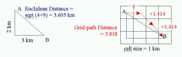
But a grid-path distance is a different matter altogether. Movement occurs from cell to cell. Following a raindrop down a slope and into a river, you’re not calculating distance as the crow flies, but in increments of one grid cell at a time, either N-S, E-W or diagonally.
Here we can see that the use of the topography as an indication of flow direction allows us to not only follow the path down slope, but we can calculate the grid-path distance as well (on a DEM layer, use r.drain).
Grid-path distance on a non-topographic surface
Suppose that movement can occur across a surface, but it occurs in response to other elements besides distance alone. Movement will be greatest where resistance or “friction” is least. This is a good description for movement of groundwater, but might also be used for disease, where resistance is inversely related to health or population density, or for animal migration where friction is a combination of factors including food, predators, climate, and topography. Movement is in inverse proportion to the “cost” of moving in any direction, and we can think of the most likely pattern of movement as being the “least-cost path.” Accumulated cost is used to define a “cost surface” and the resulting movement will be perpendicular to contours of cost, like water moving downhill perpendicular to contours.
Open the project in the “frictionQ” folder
-
- Define the cost of moving across the surface on a per cell basis. This is known as a “friction” layer or theme. The “cost” in question can be based on a numerical value or set arbitrary; for instance, I defined moving on paved road as a cost of 1, moving on dirt road as a cost of 5 (5 times slower) and moving over areas with no road as a cost of 10 (10 times slower than paved road, twice as slow as dirt road). Likewise, you can define costs by slope (steeper terrain – harder to climb), and then multiply the slope-cost & road-cost layers together, to get a holistic (but arbitrary) raster that represents friction across a surface, as a function of both road quality and steepness.
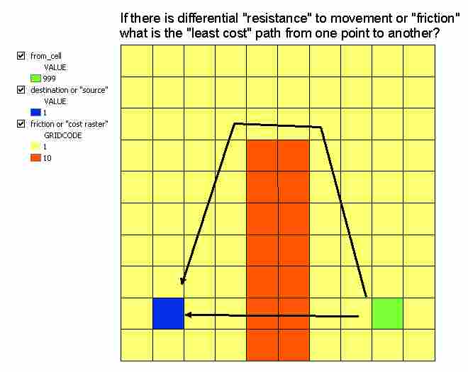
Here, the “barrier” is 10 times more costly to movement (10 times the friction) than the background. - Establish the cost surface by calculating the accumulated cost of moving from the midpoint of one cell to the midpoint of the adjacent or diagonal cell
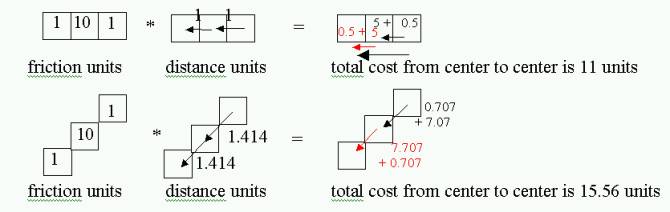 and in that way produce a “cost surface” (N.B. the output of r.cost GRASS routine does NOT include the distance, so you might consider multiplying by the distance).
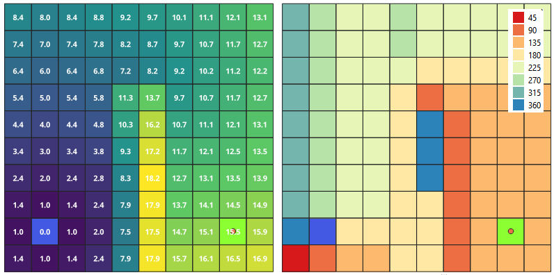
left) cost surface with values ——— right) “movement direction” map - Now we can find “least cost paths” that follow the cost surface using r.path (or alternately, usiing r.drain, which normally includes elevation plus a cost surface, and which gives slightly different results even if you leave out the elevation map.)
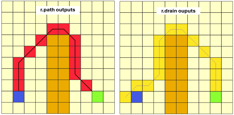
least cost paths from r.path (left) and r.drain (right)
- Define the cost of moving across the surface on a per cell basis. This is known as a “friction” layer or theme. The “cost” in question can be based on a numerical value or set arbitrary; for instance, I defined moving on paved road as a cost of 1, moving on dirt road as a cost of 5 (5 times slower) and moving over areas with no road as a cost of 10 (10 times slower than paved road, twice as slow as dirt road). Likewise, you can define costs by slope (steeper terrain – harder to climb), and then multiply the slope-cost & road-cost layers together, to get a holistic (but arbitrary) raster that represents friction across a surface, as a function of both road quality and steepness.
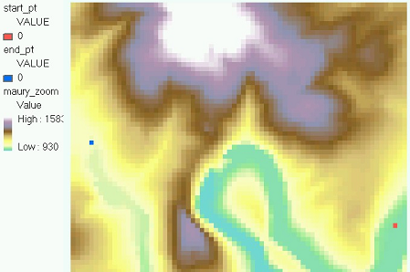
Where would you go on a hike in our topography?
If you used slope as “friction” (or squared, or cubed it), where would your “least-cost path” be from one point on a map to the next through this topography? What if you are finding a path for an animal that avoided south-facing slopes?
Dynamic Buffers (Rubber Rulers) using least-cost methods
Back to the discussion of distance maps and buffers. Can we make a dynamic buffer using cost as distance?
Imagine: How far could an exotic insect species migrate from logging trucks on major roads given its movement is a function of land use. It migrates 20 times as far or fast in the woods as in pasture/cropland, and 5 times as far in a pasture as in developed land. We can reclass the land use raster to get a cost map (see the reclass table for r.reclass called NLCD_2_friction_reclass_table.txt) using 100=urban & water; 20=ag; 1=woods
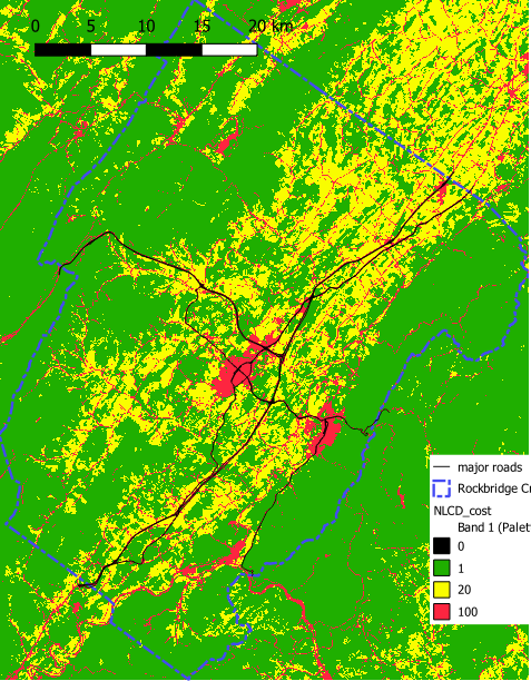
Next, executing the r.cost tool with the roads raster (1’s at road cells, null elsewhere) as “destination.” This yield a “cost surface” which could be thought as a travel time or distance of invasion map.
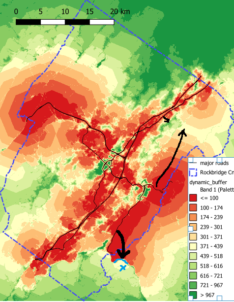
Notice how the increasing cost (which is a “distance” away) from the road and how in the NE, the travel is much longer via the Blue Ridge forest than directly from the I-81, and how the travel time suddenly increases going across the James River in the south (because water is 100 vs 1 in the forest).
Case Study (from Nick Barber’s class 2025)
-
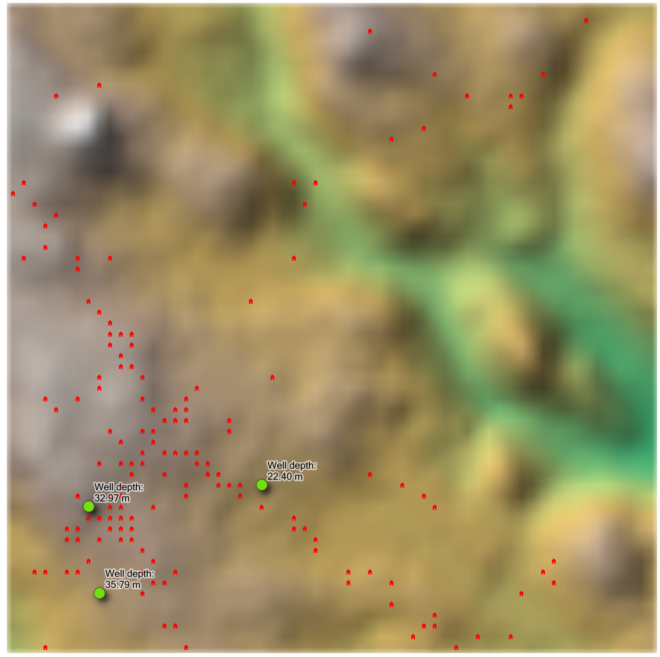
- Let’s. imagine we want to know the most efficient path, and path length, to get from homes in a mountainous area to groundwater wells (maybe we want this info to build new piping infrastructure). Note: this example comes from Hans van der Kwast.
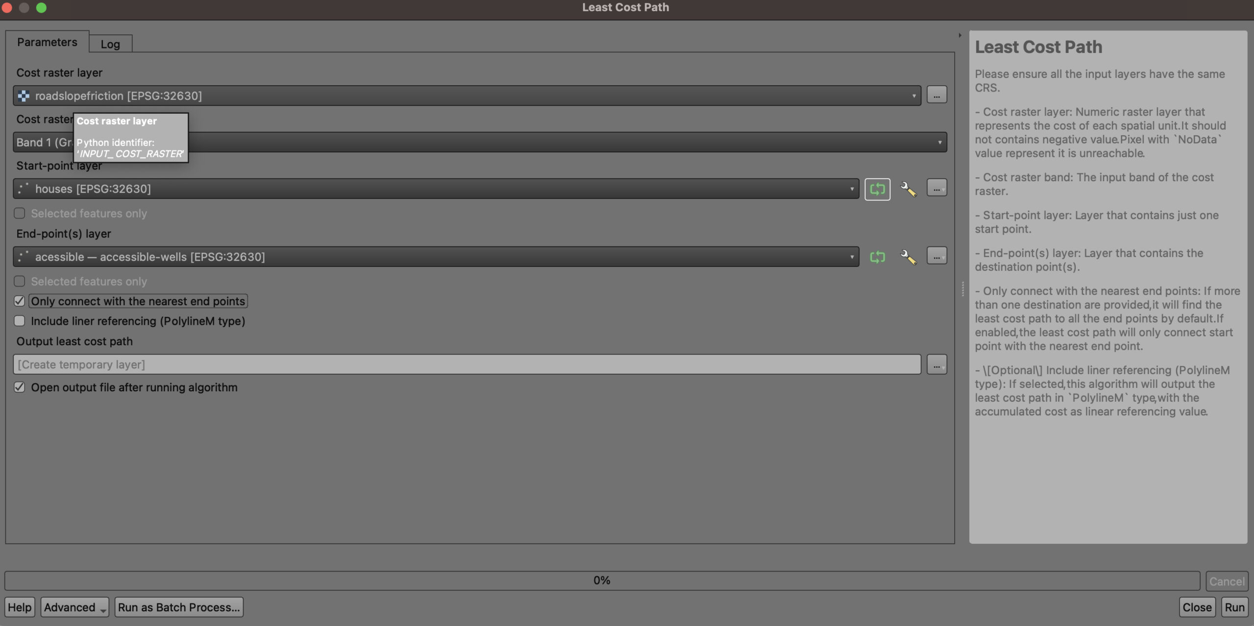
Screenshot - Now a least cost path can be made from any point (or multiple points) on the surface to the drain point on the cost surface. I used the “Least Cost Path” plugin (see here)
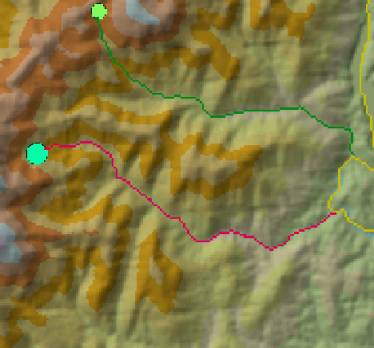
Screenshot - The resulting network looks like this (going from houses in an area to wells, over terrain and using roads as a cost surface with varying costs due to road type and slope):
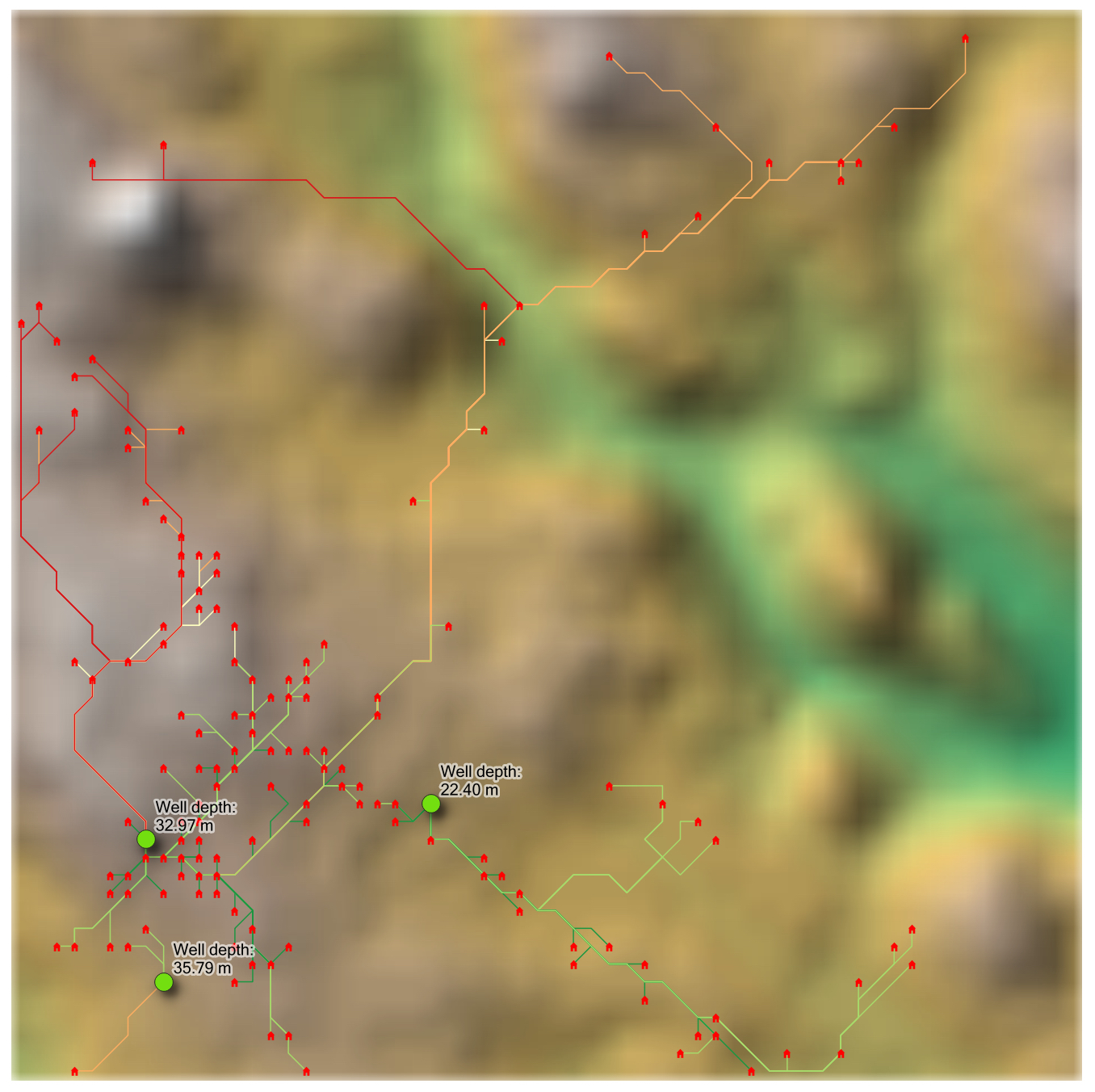
Least cost path color coded by cost distance. Despite being closer as the crow flies, some houses in the mountains have much higher costs than houses further away, because they have to travel over (1) steeper terrain; (2) less well developed roads.
- Let’s. imagine we want to know the most efficient path, and path length, to get from homes in a mountainous area to groundwater wells (maybe we want this info to build new piping infrastructure). Note: this example comes from Hans van der Kwast.