Typical spatial model developments follows the build-fit-criticize life cycle. The modeler first writes out an analogue, physical version of the model using pen and paper. Once drawn out this way, the modeler can inspect its structure and will notice any inefficiencies. Next, modeler evaluates model behavior and performance under different conditions. Such behavior is critiqued, particular with regards to speed, completeness, and robustness. This life-cycle allows the modeler to continually improve the model over time.
Simple model structure follows this scaffolding:
INPUT –> PROCESS -> OUTPUT
Such scaffolding can be layered and iterated over to produce complex, dynamic models.
See this simple example from qgis (https://docs.qgis.org/3.34/en/docs/user_manual/processing/modeler.html) 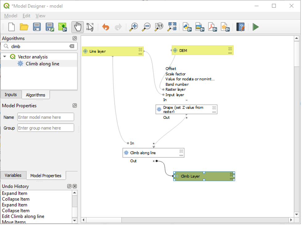
Or this simple example from ArcPro (https://pro.arcgis.com/en/pro-app/latest/tool-reference/modelbuilder-toolbox/examples-of-using-model-only-tools-in-modelbuilder.htm)

Other features of models
- Uncertainty: models with narrow “solution envelopes” (term from de Smith) have low uncertainty, but low applicability in the real world. Any good model is going to minimize uncertainty, but uncertainty needs to be quantifiable and visible in order for model to be useable.
- Error propagation problem: If there’s a 10m uncertainty in the DEM you download, that uncertainty needs to propagated through entire model
- Iteration: Models may need a “loop” structure, taking outputs and re-running them as inputs into next stage of model. Such behavior is needed with, say, climate models: if you are trying to predict global changes in sea ice over the next 50 years, your prediction 2 years from now will depend on your prediction 1 year from now.
- Stochastic behavior: Whether through empirical knowledge or numerical modeling, natural processes involve a degree of “randomness” that is useful to include in spatial models. Consider a wildfire model – without advanced knowledge of lightning strikes or arson events (and if you have such prior knowledge…I am suspicious of your after school activities), the starting location of any such spatial model is to some extent, random, within thee confines of the parameters that drive wildfires
See as an example if iterative & stochastic modeling, the USDA FlamMap model

Input data themes required for running FlamMap are the same as those for FARSITE and are contained in a “Landscape” file constructed from ASCII Grid fi les that are of identical resolution, co-registered, and of equal extent. Adapated from Finney (2006)
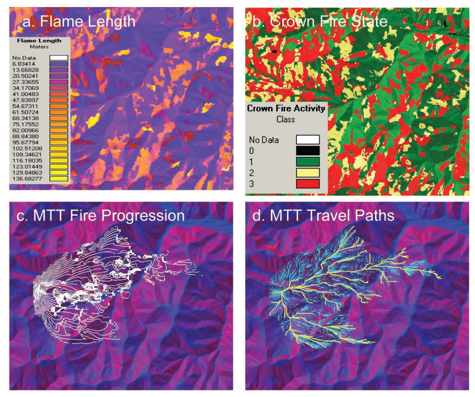
Example outputs from FlamMap: a) fire spread rate, (b) crown fire activity (0=none, 1=surface fire, 2=torching trees or passive crown fire, and 3=active crown fire), (c) fire progression (white perimeters) simulated using the Minimum Travel Time (MTT) method, and (d) the fire travel paths produced by MTT (bold yellow lines distinguish major paths from all paths in light blue). Adapated from Finney 2006
Some important decisions we have to make as modelers: what solution envelope (range of solutions) do I want?
Decision we make as modelers can only be justified based on prior knowledge, existing data, and physical parameters of the problem we are trying to solve.
Limitations on our modeling workflow:
- Availability of inputs needed to accomplish task i.e., is relevant data publicly available, or available in the right data format?
- Our knowledge of the problem as a user. If I ask you to build a volcano hazard model, most of you will struggle to know where to start
- *Computer resources*
- Models are computationally expensive especially dynamic, iterative models
- Poorly designed models will take too long to run
- In modeling, time is $$